![]()
![]()
| Part 1 | Part 2 | Live Demo | References |
![]()
Shaders are 'small' program
executed directly in the GPU. With shaders, we have the possibility to program
the OpenGL pipeline to implement our own light model, mapping, shadowing ...
This project will talk about some rendering techniques implemented using GLSL
shaders (OpenGl Shading Language). In the first part, I will present some
advanced rendering mapping techniques. The second part is dedicated to more
common shaders, which are integrated in the Bonzai Engine.
So, lets begin with the most interesting stuff: advanced per-pixel rendering mapping
techniques. To introduce this, I will present you first the normal mapping (also
known as dot3 bump mapping). Then, I will present you some impressive results
achieved with some more advanced techniques.
This page is intended to introduce you the abilities of recent graphic cards
with some impressive results of state of the art rendering techniques, instead
than to detail you how each techniques works. For people interested in learning
more, read the great technical papers listed at the end of the document. They
are really fantastic !
I let you read by your own the glsl code available in Bonzai Engine
(and the Model Viewer) and the tangent space
lesson.
If you have any question, don't hesitate to contact me either via my
mail or the forum.
Great reading !
Shaders are highly dependant of the graphic card capabilities.
From a graphic
card to another, they can be a high difference from the hardware that limits
implementation of some rendering algorithms (expecially comparing recent and not
so recent cards).
For example, my old desktop's graphic card, a Radeon 9600 Pro, have too many
limitations that make practically impossible to run the the shaders based on
parallax algorithm corrections with iteration. Here
are few limitations of that graphic card: for/while statement not supported, 96 instructions limit, 64 arithmetic operations limit ...
I've bought recently an NVidia 7600 GS graphic card which support pixel shader
3.0. The shader you'll find at the end of the document was written and executed
on that graphic card.
Shaders are used to implement advanced rendering technique such as per pixel
lighting, normal mapping (bump), parallax mapping ...
Here is a screenshot of a model rendered with per pixel light and normal mapping
(per pixel normal perturbation) :
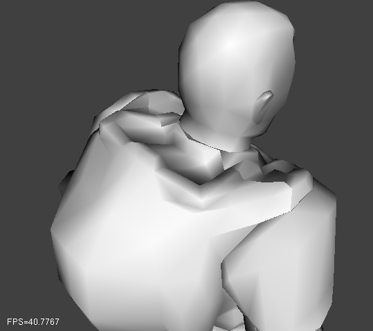
Per vertex lighting (classic rendering)
![]()
Per pixel lighting + Normal mapping
You can see the huge difference between classic rendering (ie default per vertex
lighting model) with a per pixel lighting with normal perturbation.
The geometry used to render these pictures is the same (ie same number of
polygons). Normal mapping perturbates normal at each pixel. With the use of a
per pixel lighting, the behavior of surface illuminating is modified. In the following
picture, pixel normals are displayed as rgb color (normal.x is read, ...) :
![]()
Pixel normal perturbation
I will present you some results obtained with different rendering techniques
based on texture coordinate correction for adding some height on planar surface.
In all following screenshots, the shape drawn is a planar surface made of just 4
vertices. Diffuse texture is disable for a better comparison.
Parallax mapping with offset limiting
I've implemented this technique thanks to the great article
Parallax Mapping with Offset Limiting: A PerPixel
Approximation of Uneven Surfaces written by
Terry Welsh.
To know more about this technique, read this article.
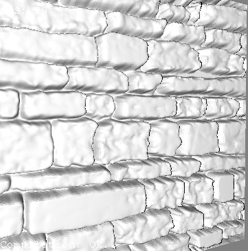
I will present you results of the present rendering technique on a quad shape.
The base is a quad with normal mapping, you can note a slite depth effect added
thanks to this rendering technique presented previously.
Normal mapping on a flat quad
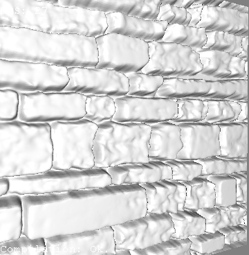
Now the result using this parallax technique from the same view point.
This technique gives great results of this technique at such view position. This
create an amplified depth effect compared to the classic normal mapping
technique.
You can notice a small rendering artifact on the first picture, which is slitly
reduced in the second.
|
|
|
|
Normal mapping |
Normal mapping |
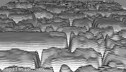
Now, what is the result for close-up view ?
A close-up view on this quad rendered with normal mapping :
Normal mapping
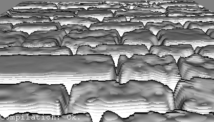
For close-up view, this technique make really bad results (first picture).
By using it in multiple step (3 times for the second picture), the quality
obtain can be improved a lot.
 |
 |
|
Normal mapping |
Normal mapping |
Depth scaling is 0.05, upper scaling value makes lot more artifacts. No bias is applied (don't yet tried it but for what I read this can
improved the rendering quality especially on close-up view).
This technique is appropriate for small displacement. For higher displacement more
advanced/complicated techniques should be used. I think, in general, the scaling
limit is about 0.03 especially if no bias is applied.
TODO: Try with bias offset.
Those three rendering techniques are based on a linear/binary search to find the height
of each pixels (of the primitive polygon). The implementation of these techniques are based on those very
impressive papers :
Steep Parallax Mapping,
written by Morgan McGuire & Max McGuire
Iterative Parallax Mapping
with Slope Information, written by
Matyas Premecz
Real-Time Relief Mapping on
Arbitrary Polygonal Surfaces, written by Manuel M. Oliveira
& Fabio
Policarpo
An Efficient Representation
for Surface Details, written by Fabio
Policarpo & Manuel M. Oliveira
IMPORTANT NOTE :
THE RESULTS PRESENTED HERE ARE BASED ON MY IMPLEMENTATION OF THESE
TECHNIQUES. IMPLEMENTATION ARE NOT FULLY COMPLETE AND RESULT CAN SURELY BE
IMPROVED. PAPER'S AUTHOR HAVE BETTER RESULTS THAN THOSE PRESENTED UNDERNEATH.
SOME AUTHOR USES TEXTURE BIAS WHICH SEEM TO IMPROVE A LOT THE RENDERING.
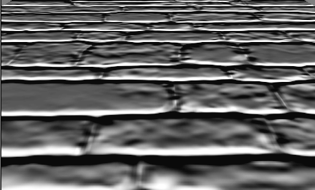
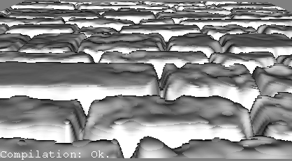
For such view point, these three techniques gives the same results. Height
factor used is 0.1 and 14 iterations are performed for avery vertices. Notice
the higher height created by those techniques compared to the basic parallax
mapping technique.
 |
 |
 |
|
Steep Parallax Mapping |
Relief Mapping 10 linear iterations 4 binary iterations |
Iterative Parallax Mapping |
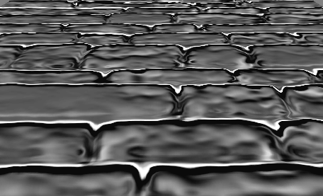
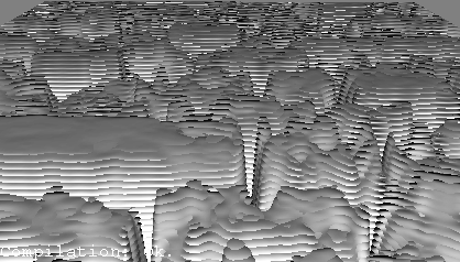
For close-up view, you can notice the steps of the linear/binary search.
Steep parallax gives bad results, relief mapping have medium quality. Iterative
mapping is the fastest converging technique and give really good results on this
example, even at distant points.
Height factor used is 0.1 and 14 iterations was performed for every pixels.
 |
 |
 |
|
Steep Parallax Mapping |
Relief Mapping 10 linear iterations 4 binary iterations |
Iterative Parallax Mapping |
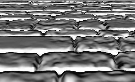
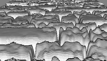
In the following screenshots, the view point is the same. The height factor is
changed to 0.2 for higher depth, number of iterations is also increased.
Iterative mapping give great results for those settings. The two other
techniques requieres more iteration to obtain equivalent rendering quality.
 |
 |
 |
|
Steep Parallax Mapping |
Relief Mapping 20 linear iterations 5 binary iterations |
Iterative Parallax Mapping |
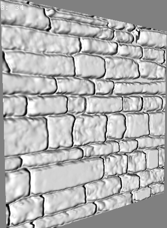
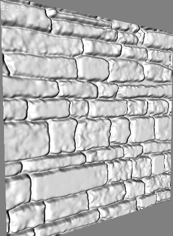
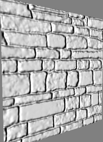
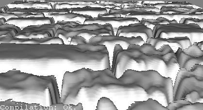
Here are some animations showing iterative mapping in action :
 |
 |
|
Iterative mapping height factor of 0.1 10 linear iterations 4 binary iterations |
Iterative mapping |
Iterative mapping
height factor of 0.1
10 linear iterations
4 binary iterations
Iterative mapping
height factor of 0.1
20 linear iterations
4 binary iterations
Iterative mapping
height factor of 0.05
10 linear iterations
4 binary iterations
TODO: Try with bias offset.
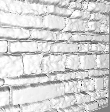
In the 3 previous techniques, when too small iterations was performed,
iterations steps are visible. The two rendering techniques presented here are
some optimization of previous techniques to avoid this rendering artefact.
The implementation of these techniques are based on those very impressive papers
:
Interval Mapping,
written by Eric Risser, Musawir Shah & Sumanta
Pattanaik
Practical Parallax Occlusion
Mapping, written by
Natalya Tartachuk
TO BE WRITTEN
By reading the Parallax Occlusion paper, I've remaked that a piece of code can
be optimize for the calculation of
vParallaxOffsetTS
(you'll save approximatively 9 ALU operations, Arithmetic Logic Unit).
The result is of course exactly the same, and you'll see the code is cleanier
and easier to understand. If you're interested, here is the original vertex
code and *optimized* vertex code.
Original vertex code |
// Compute the ray direction
for intersecting the height field profile with |
New Vertex code |
// Compute the ray direction
for intersecting the height field profile with |
All previous rendering technique are working on TBN (Tangent Binormal Normal)
space. To know what is TBN space and how to calculate TBN vectors/matrix, look
at lesson 8.
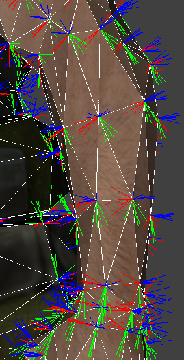
The TBN space is calculated for a face and depends on the face vertices and
textures coordinates. The results of this calculation is displayed in the first
screenshot below. The model is drawn in solid and wire mode to display
explicitly face boundaries. For each face vertex, the TBN vectors are drawn. As
face share vertices, on a particular vertices, TBN vectors will be drawn more
than one time.
You can notice a flat transition between face TBN vectors.
To obtain a smooth transition, we average TBN vectors (the calculation is
equivalent to passing from per face normal to per vertex normal). You can notice
on the second screenshot that the TBN space is the same on a vertice,
independently from the face it belongs.
 |
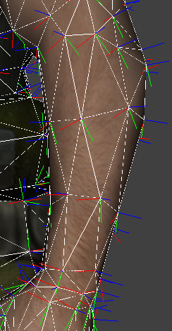 |
| Per face TBN |
Per vertex TBN |
T is displayed in red
B is displayed in green
N is displayed in blue
Remark: The view point is slightly different between the two screenshots.
If you're interested in GLSL shader code used for rendering the screenshot
above, look at the Bonzai Engine
projects.
All the algorithms presented here, and on the second part
of the document, has been integreted inside the Bonzai Engine, which is
used by the Model Viewer.
With the model viewer, associated with the demo models, can be used to get and/or
edited GLSL shaders. Go to the
download section to get them (a login may be requiered for downloading the demo models,
but you can use your own models).
Basics steps for that is: open any 3D models, go to Render->Shader Config.
Loads the GLSL shaders by unchecking Auto-generate button and select a
preset . They will be shown on the model tree (advanced tree mode), double click
on a shader and the shader editor panel will the vertex and fragment glsl source
code.
If you still have questions, you can contact me via my
mail or the forum.
Steep Parallax Mapping
written by Morgan McGuire & Max McGuire
Iterative Parallax Mapping
with Slope Information
written by
Matyas Premecz
Real-Time Relief Mapping on
Arbitrary Polygonal Surfaces
written by Manuel M. Oliveira and Fabio
Policarpo
An Efficient Representation
for Surface Details
written by Fabio
Policarpo & Manuel M. Oliveira
Interval Mapping
written by Eric Risser, Musawir Shah & Sumanta
Pattanaik
Practical Parallax Occlusion
Mapping
written by
Natalya Tartachuk
Note: All those papers are available on the web,
just make a search on the web with your favorite search engine and you will find them
very easily.
![]()
| Last modified on 01/07/2010 | |
| Copyright © 2004-2012 JĂ©rĂ´me JOUVIE - All rights reserved. | http://jerome.jouvie.free.fr/ |